5.2 JSON data

Data provided via web APIs is often made available in JSON (JavaScript Object Notation) format, a simple human readable text format for storing hierarchical data.

There are a few R packages that parse JSON data, but jsonlite is our package of choice. Like readr and sf, jsonlite can read data directly from a URL.

Data for for the following examples is sourced from the Australian Bureau of Meteorology’s Latest Weather Observations for Melbourne Airport, made available directly from their website in JSON format.

# Bureau of Meteorology - Latest Weather Observations for Melbourne Airport
bom_url <- "http://www.bom.gov.au/fwo/IDV60901/IDV60901.94866.json"

bom_data <- jsonlite::fromJSON(bom_url)

jsonlite has an intuitive mapping from JSON data types to R. The object returned from the BoM site is a list containing various pieces of metadata alongside our data of interest.

Check out the original URL to see the JSON data that has been mapped to this R structure.

str(bom_data)
#> List of 1
#>  $ observations:List of 3
#>   ..$ notice:'data.frame':   1 obs. of  4 variables:
#>   .. ..$ copyright     : chr "Copyright Commonwealth of Australia 2020, Bureau of Meteorology. For more information see: http://www.bom.gov.a"| __truncated__
#>   .. ..$ copyright_url : chr "http://www.bom.gov.au/other/copyright.shtml"
#>   .. ..$ disclaimer_url: chr "http://www.bom.gov.au/other/disclaimer.shtml"
#>   .. ..$ feedback_url  : chr "http://www.bom.gov.au/other/feedback"
#>   ..$ header:'data.frame':   1 obs. of  8 variables:
#>   .. ..$ refresh_message: chr "Issued at  2:11 pm EDT Tuesday  1 December 2020"
#>   .. ..$ ID             : chr "IDV60901"
#>   .. ..$ main_ID        : chr "IDV60900"
#>   .. ..$ name           : chr "Melbourne Airport"
#>   .. ..$ state_time_zone: chr "VIC"
#>   .. ..$ time_zone      : chr "EDT"
#>   .. ..$ product_name   : chr "Capital City Observations"
#>   .. ..$ state          : chr "Victoria"
#>   ..$ data  :'data.frame':   161 obs. of  35 variables:
#>   .. ..$ sort_order          : int [1:161] 0 1 2 3 4 5 6 7 8 9 ...
#>   .. ..$ wmo                 : int [1:161] 94866 94866 94866 94866 94866 94866 94866 94866 94866 94866 ...
#>   .. ..$ name                : chr [1:161] "Melbourne Airport" "Melbourne Airport" "Melbourne Airport" "Melbourne Airport" ...
#>   .. ..$ history_product     : chr [1:161] "IDV60901" "IDV60901" "IDV60901" "IDV60901" ...
#>   .. ..$ local_date_time     : chr [1:161] "01/02:00pm" "01/01:30pm" "01/01:00pm" "01/12:30pm" ...
#>   .. ..$ local_date_time_full: chr [1:161] "20201201140000" "20201201133000" "20201201130000" "20201201123000" ...
#>   .. ..$ aifstime_utc        : chr [1:161] "20201201030000" "20201201023000" "20201201020000" "20201201013000" ...
#>   .. ..$ lat                 : num [1:161] -37.7 -37.7 -37.7 -37.7 -37.7 -37.7 -37.7 -37.7 -37.7 -37.7 ...
#>   .. ..$ lon                 : num [1:161] 145 145 145 145 145 ...
#>   .. ..$ apparent_t          : num [1:161] 18.8 17.3 15.3 14 14.1 14.2 13.9 15.6 17.5 19.4 ...
#>   .. ..$ cloud               : chr [1:161] "Mostly clear" "Mostly clear" "Mostly clear" "Cloudy" ...
#>   .. ..$ cloud_base_m        : int [1:161] 600 600 600 3300 3300 2610 2500 1110 1110 2340 ...
#>   .. ..$ cloud_oktas         : int [1:161] 1 1 1 8 8 3 8 1 1 3 ...
#>   .. ..$ cloud_type_id       : int [1:161] 6 6 6 NA NA NA 35 6 6 NA ...
#>   .. ..$ cloud_type          : chr [1:161] "Stratocumulus" "Stratocumulus" "Stratocumulus" "-" ...
#>   .. ..$ delta_t             : num [1:161] 4.5 4 3.2 2.7 2.8 3.3 3.6 7.5 7.4 7.7 ...
#>   .. ..$ gust_kmh            : int [1:161] 33 33 39 39 37 52 52 59 50 59 ...
#>   .. ..$ gust_kt             : int [1:161] 18 18 21 21 20 28 28 32 27 32 ...
#>   .. ..$ air_temp            : num [1:161] 21.7 20.4 19.4 18.5 18.6 19.3 19.5 23.1 24.2 25 ...
#>   .. ..$ dewpt               : num [1:161] 14 13.5 13.9 13.8 13.7 13.6 13.2 9.3 11.1 11.5 ...
#>   .. ..$ press               : num [1:161] 1005 1006 1005 1004 1004 ...
#>   .. ..$ press_qnh           : num [1:161] 1006 1006 1005 1005 1005 ...
#>   .. ..$ press_msl           : num [1:161] 1005 1006 1005 1004 1004 ...
#>   .. ..$ press_tend          : chr [1:161] "-" "-" "-" "-" ...
#>   .. ..$ rain_trace          : chr [1:161] "0.0" "0.0" "0.0" "0.0" ...
#>   .. ..$ rel_hum             : int [1:161] 61 64 70 74 73 69 67 41 43 42 ...
#>   .. ..$ sea_state           : chr [1:161] "-" "-" "-" "-" ...
#>   .. ..$ swell_dir_worded    : chr [1:161] "-" "-" "-" "-" ...
#>   .. ..$ swell_height        : logi [1:161] NA NA NA NA NA NA ...
#>   .. ..$ swell_period        : logi [1:161] NA NA NA NA NA NA ...
#>   .. ..$ vis_km              : chr [1:161] "10" "10" "10" "10" ...
#>   .. ..$ weather             : chr [1:161] "-" "-" "-" "Showers" ...
#>   .. ..$ wind_dir            : chr [1:161] "N" "NNW" "N" "NNE" ...
#>   .. ..$ wind_spd_kmh        : int [1:161] 22 22 28 30 30 33 35 39 37 32 ...
#>   .. ..$ wind_spd_kt         : int [1:161] 12 12 15 16 16 18 19 21 20 17 ...

JSON data is often hierarchically structured or nested in this way, and you’ll need to work your way through the structure to get to the data you need.

class(bom_data)
#> [1] "list"
names(bom_data)
#> [1] "observations"
names(bom_data$observations)
#> [1] "notice" "header" "data"

class(bom_data$observations$data)
#> [1] "data.frame"
bom_data$observations$data %>% as_tibble()
#> # A tibble: 161 x 35
#>    sort_order   wmo name  history_product local_date_time local_date_time…
#>         <int> <int> <chr> <chr>           <chr>           <chr>           
#>  1          0 94866 Melb… IDV60901        01/02:00pm      20201201140000  
#>  2          1 94866 Melb… IDV60901        01/01:30pm      20201201133000  
#>  3          2 94866 Melb… IDV60901        01/01:00pm      20201201130000  
#>  4          3 94866 Melb… IDV60901        01/12:30pm      20201201123000  
#>  5          4 94866 Melb… IDV60901        01/12:27pm      20201201122700  
#>  6          5 94866 Melb… IDV60901        01/12:03pm      20201201120300  
#>  7          6 94866 Melb… IDV60901        01/12:00pm      20201201120000  
#>  8          7 94866 Melb… IDV60901        01/11:37am      20201201113700  
#>  9          8 94866 Melb… IDV60901        01/11:30am      20201201113000  
#> 10          9 94866 Melb… IDV60901        01/11:14am      20201201111400  
#> # … with 151 more rows, and 29 more variables: aifstime_utc <chr>, lat <dbl>,
#> #   lon <dbl>, apparent_t <dbl>, cloud <chr>, cloud_base_m <int>,
#> #   cloud_oktas <int>, cloud_type_id <int>, cloud_type <chr>, delta_t <dbl>,
#> #   gust_kmh <int>, gust_kt <int>, air_temp <dbl>, dewpt <dbl>, press <dbl>,
#> #   press_qnh <dbl>, press_msl <dbl>, press_tend <chr>, rain_trace <chr>,
#> #   rel_hum <int>, sea_state <chr>, swell_dir_worded <chr>, swell_height <lgl>,
#> #   swell_period <lgl>, vis_km <chr>, weather <chr>, wind_dir <chr>,
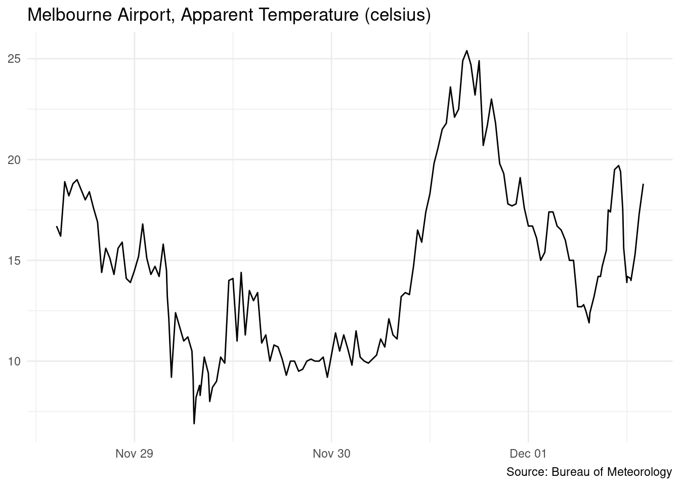
#> #   wind_spd_kmh <int>, wind_spd_kt <int>

Just for fun, here’s the temperature as a line graph.

library(ggplot2)
bom_data$observations$data %>%
  ggplot(aes(x = lubridate::as_datetime(local_date_time_full), y = apparent_t)) +
  geom_line() +
  theme_minimal() +
  theme(legend.position = "bottom",
        axis.title = element_blank(),
        legend.title = element_blank()) +
  labs(title = "Melbourne Airport, Apparent Temperature (celsius)",
       caption = "Source: Bureau of Meteorology")